Separable Differential Equations

Introduction

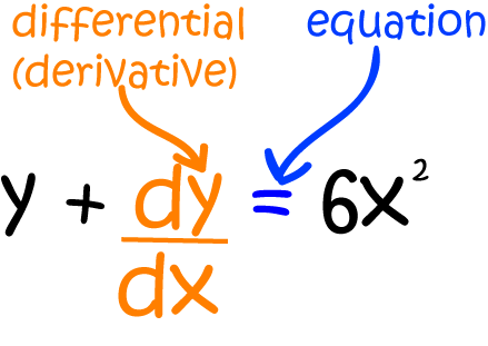
Differential Equations are equations involving a function and one or more of its derivatives.

For example, the differential equation below involves the function \(y\) and its first derivative \(\dfrac{dy}{dx}\).

Let's consider an important real-world problem that probably won't make it into your calculus text book:

A plague of feral caterpillars has started to attack the cabbages in Gus the snail's garden. Gus observes that the cabbage leaves are being eaten at the rate

where \(t\) is the time in days after the initial infestation. He knows that \(6\) cabbage leaves were eaten during the initial infestation, and wants to know how many cabbage leaves will be eaten on the first day after the infestation.
Gus has written down a separable differential equation. This means that we can split it up to pull all the parts of the equation involving \(\text{cabbage}\) onto one side of the equation, and the parts of the equation involving \(t\) onto the other side of the equation: To work out how many cabbage leaves will be eaten on day \(1\), he needs to solve his differential equation and plug in \(t= 1\). But how can he solve the equation? Separable differentiable equations are one of the easiest types of differential equations to solve. We solve them using a method called separation of variables. It only works for separable differential equations like this one.

Separation of Variables

Solving differential functions involves finding a single function, or a collection of functions that satisfy the equation.

Separable differential equations are one class of differential equations that can be easily solved. We use the technique called separation of variables to solve them.

For example, the differential equation

is a separable differential equation:

Steps in the Method

The method of separation of variables involves three steps:

1. Move all the terms in \(y\), including \(dy\), to one side of the equation and all the terms in \(x\), including \(dx\), to the other.
2. Integrate both sides: the \(y\)-side with respect to \(y\), and the \(x\)-side with respect to \(x\).
3. Simplify your equation.

That sounds fair enough, doesn't it? Let's see it in action:

Example:

Solve the equation

using separation of variables.

Step 1: Separate the variables by moving all the terms in \(y\), including \(dy\), to one side of the equation and all the terms in \(x\), including \(dx\), to the other.

Step 2: Integrate both sides of the equation.

Step 3: Simplify the equation (get rid of the log by taking exponentials of each side).

So, the solution is

Example (Fruit flies)

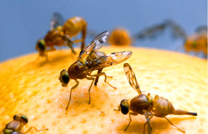You've probably encountered fruit flies before. They're the pesky little things that seem to materialise out of thin air and buzz around the stoned fruit in the summer. Biologists are interested in fruit flies because they breed quickly and easily, and are useful for exploring the transmission of genetic traits.

Biologists are also interested in modelling the growth of populations, and fruit fly populations certainly grow! You need fruit flies to produce more fruit flies, and as you get more fruit flies, the fruit fly population increases more and more rapidly. So, if I want to model the growth of the fruit fly population in and around my fruit bowl, I need to come up with some parameters (variables) for my model. I think the following will be helpful:

• The time, \(t\).
• The number of fruit flies present and any time \(t\). Let's call it \(F\).
• The rate of change of the fruit fly population, \(\dfrac{dF}{dt}\).

My fruit fly population is constantly, annoyingly, increasing, and I want to model its growth at any time. The rate of change (at any time) of the fruit fly population is equal to the population's growth rate times the number of fruit flies present at that time, so we can set up the following differential equation:

The above equation is a separable differential equation, so we can solve it using separation of variables. It doesn't matter that the variable names are different. We can use the method anyway.

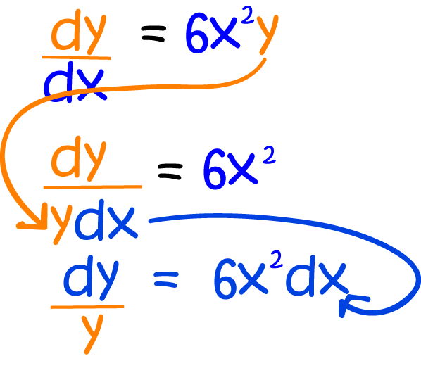
Step 1: Separate the variables by moving all the terms in \(F\), including \(dF\), to one side of the equation and all the terms in \(t\), including \(dt\), to the other.

Step 2: Integrate both sides of the equation.

Step 3: Simplify the equation (get rid of the log by taking exponentials of each side).

So, the solution is (drum roll, please) ... : Here, \(A\) and \(k\) are constants.

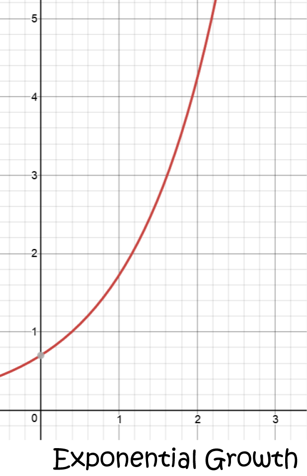
Just for fun, let's choose some values of \(A\) and \(k\), say \(A = 0.7\), and \(k = 0.9\), and have a look at the graph:

Note: The differential equation in this example crops up all over the place when we're modeling the growth of populations or investments, or things like radioactive decay. In fact, Gus' differential equation has this type. Let's solve it!

Solving Gus' Feral Caterpillar Problem

If you recall, Gus' garden has been infested with caterpillars, and they are eating his cabbages. He's modelled the situation using the differential equation:

where \(t\) is the time in days after the initial infestation. He knows that \(6\) cabbage leaves were eaten during the initial infestation, and wants to know how many cabbage leaves will be eaten on day \(1\). He needs to solve the differential equation, work out the value of \(A\), and plug in \(t = 1\).

Well, the first step has already been done for us. If we plug \(F = \text{cabbage}\) and \(k = 5\) into the above equation, we get Gus' equation, and its solution is

So, now we need to find the value of \(A\). We're told that \(6\) cabbage leaves were eaten during the initial infestation. This is an example of an initial condition and we can use it to find the value of \(A\). Plug \(t = 0\) and \(\text{cabbage} = 6\) into our equation to give: That was easy! So, now we have the particular solution of Gus' equation that he requires: We can plug in \(t = 1\) to find out how many leaves were eaten on day \(1\) after the infestation: That's a lot of cabbage. No wonder Gus is so worried!

Some More Examples

Let's finish with three more examples. Each of them will be slightly harder than the previous one, so it's a good idea to look at them in order.

Example 1

Solve the differential equation \(\dfrac{dy}{dx} = \dfrac{1}{y^2}\).

At first glance, this doesn't look like a separable differential equation (there's no \(x\), but it is (the function of \(x\) is just the constant function, \(1\)). Let's separate away:

Step 1: Separate the variables by moving all the terms in \(x\), including \(dx\), to one side of the equation and all the terms in \(y\), including \(dy\), to the other.

Step 2: Integrate both sides of the equation.

Step 3: Simplify the equation:

Note: You need to be careful with constants and differential equations. This solution is not the same as \(y = \sqrt[3]{3x} + C\). We need to add the constant during integration, not at the end of the procedure.

Example 2

Solve the differential equation \(\dfrac{dy}{dx} = \dfrac{3x^2 y}{4 + x^3}\).

This one is definitely separable. Let's set to work:

Step 1: Separate the variables by moving all the terms in \(x\), including \(dx\), to one side of the equation and all the terms in \(y\), including \(dy\), to the other.

Step 2: Integrate both sides of the equation.

The left hand side is just \(\ln |y|\). We'll need to use integration by substitution to integrate the right hand side:
Let \(u = 4 + x^3\). Then \(du = 3x^2 \; dx\). So, we have

Step 3: Simplify the equation:
There's no more work to be done, so the solution is

Example 3: The Verhulst Equation and the Carrying Capacity of Environments

Back to Our Fruit Flies

Our original model for the rate of change of the fruit fly population wasn't quite realistic enough because it failed to take into account the fact that a given environment (like my fruit bowl) only has enough food in it to support a certain population. This maximum population that an environment can support is called the carrying capacity of the environment.

A Belgian mathematician, Pierre Francois Verhulst, figured this out in 1838, and his work was later modified by American scientists Raymond Pearl and Lowell Reed to produce the Verhulst equation:

in which \(P(t)\) represents the population at time \(t\), \(r\) is the growth rate and \(K\) is the carrying capacity of the environment. Pretty clever, huh?

Let's write it using the variable names we had before:

where \(F(t)\) is the fruit fly population at time \(t\), \(k\) is the growth rate, and \(K\) is the carrying capacity of the fruit bowl environment.

This equation can be solved using the separation of variables method, but we need to get a bit tricky:

Step 1: Separate the variables by moving all the terms in \(F\), including \(dF\), to one side of the equation and all the terms in \(t\), including \(dt\), to the other. We'll do this in two stages:

Step 2: Integrate both sides of the equation. We'll need to work on the left hand side a little first using partial fractions.

Now, it's much easier to integrate. Let's hop to it (fly to it, perhaps?)

Step 3: Simplify the equation. There are more sneaky tricks to come!

We could leave it there, but it doesn't look very pretty. We want to get \(F\) on its own as the subject of the formula.

Time for some more sneaky algebra tricks!

Phew, that was a bit of a marathon! So, our solution is

Let's see what it looks like with \(K = 30\), \(A = 7\), and \(k = 3\):

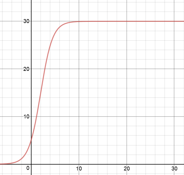
\(K\) is on the vertical axis and \(t\) is on the horizontal axis. The graph initially rises like an exponential function, but then flattens out as \(K\) gets closer to \(30\).