Calculus
Chapters
Integrals and Approximations
Integrals and Approximations
The tool of choice for finding the area under a curve is integration. Most of the time, integration gives us an exact answer for the area.
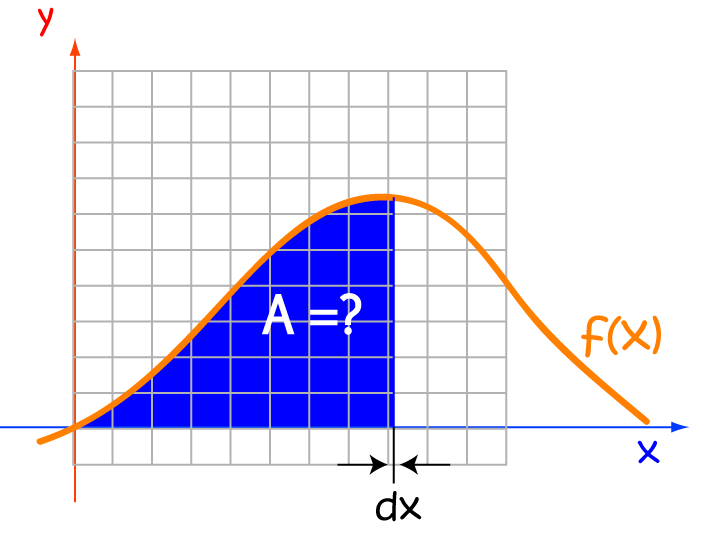
Unfortunately, there are times when integration just can't help us out. Some integrals are very difficult to find. Other functions, such as \(f(x) = e^{x^2}\) have no anti-derivative. Sometimes, we don't even know what a function is, but we still need to find the area under its curve.
Fortunately, there are a number of integral approximation techniques that can help us out. Although they can't give us an exact answer, they can give us an approximation, and that is often good enough. Some of these techniques just involve adding up lots of rectangles that have been drawn at various points under the curve. We can improve their accuracy by using smaller rectangles. There are also formulas which let us calculate the maximum errors in these approximations. This can be very helpful for engineers, for example, who really need to avoid having their buildings and bridges tumble down. Let's explore some of the techniques for approximating integrals that are available.
Examples
We're going to test out five integral approximation techniques on the definite integral of the function \(f(x) = \ln (x)\) from \(x = 1\) to \(x = 5\). This is a nice, friendly, function that has an antiderivative of \(x \ln x - x\), and we can evaluate the definite integral to get the exact answer of \(4.04718956210502\dots\). Because of this, we have a great basis for comparing the accuracy of each of the five approximation techniques that we're interested in. Let's now forget that we ever knew how to integrate \(\ln(x)\). Each of our integration techniques will require us to find some function values. We'll put most of these in a table so that we can refer back to them at any time.
| \(x\) | \(\ln(x)\) |
|---|---|
| \(1\) | \(0\) |
| \(2\) | \(0.6931471806\dots\) |
| \(3\) | \(1.098612289\dots\) |
| \(4\) | \(1.386294361\dots\) |
| \(5\) | \(1.609437912\dots\) |
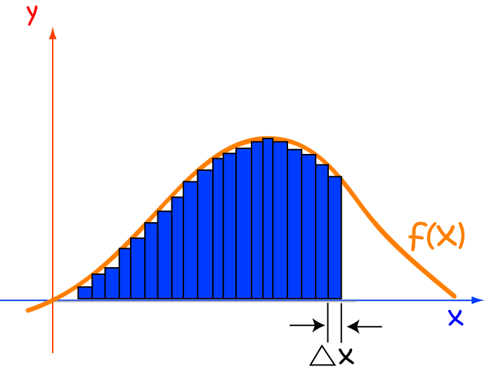
Each approximation method will require us to decide on the size of the chunks that we want to break the interval \([1,5]\) up into.
Another term for this is the slice width, you might be asked for the number of function values, the number of sub-intervals, or
the number of subdivisions. We're going to make
the simplest choice: each slice will have width \(1\). However, bear in mind that taking smaller slice widths leads to better approximations, which is a good
thing!
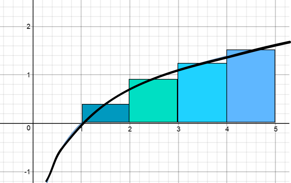
Left Rectangular Approximation Method (LRAM)
This method is also known as finding the Left Riemann Sum. Funnily enough, this method approximates the area under our curve using
rectangles. The heights of these rectangles are equal to the function values at the left hand end points of each slice, and their widths are equal to
the slice width we chose. Have a look at the picture below to get a better idea of what's going on.
 .
.
We need to find the areas of each of the \(4\) rectangles in the picture and add them together. This will be our Left Riemann Sum, and
integral approximation. Oh, and by the way, I saw that look you gave me earlier: there are \(4\) rectangles! The left-most one has height zero, so you're
forgiven for not noticing it.
Let's calculate the areas of those rectangles:
| \(x\)-values | Area Calculation | Area of Rectangle |
|---|---|---|
| 1 - 2 | \(\ln(1) \times 1\) | \(0 \times 1 = 0\) |
| 2 - 3 | \(\ln(2) \times 1\) | \(0.6931471806\dots\) |
| 3 - 4 | \(\ln(3) \times 1\) | \(1.098612289\dots\) |
| 4 - 5 | \(\ln(4) \times 1\) | \(1.386294361\dots\) |
Adding these together gives a LRAM approximation of \(3.1780538303\dots\). This is much lower than the actual value of the integral, and if you look at the picture of the rectangles, you can see why. There's quite a big gap between the tops of each rectangle and the curve.
Note: Left Riemann Sums will always provide under-estimates for areas under increasing curves. If the curve does some to-ing and fro-ing between increasing and decreasing, some of these errors will cancel each other out, and the approximation will be better.
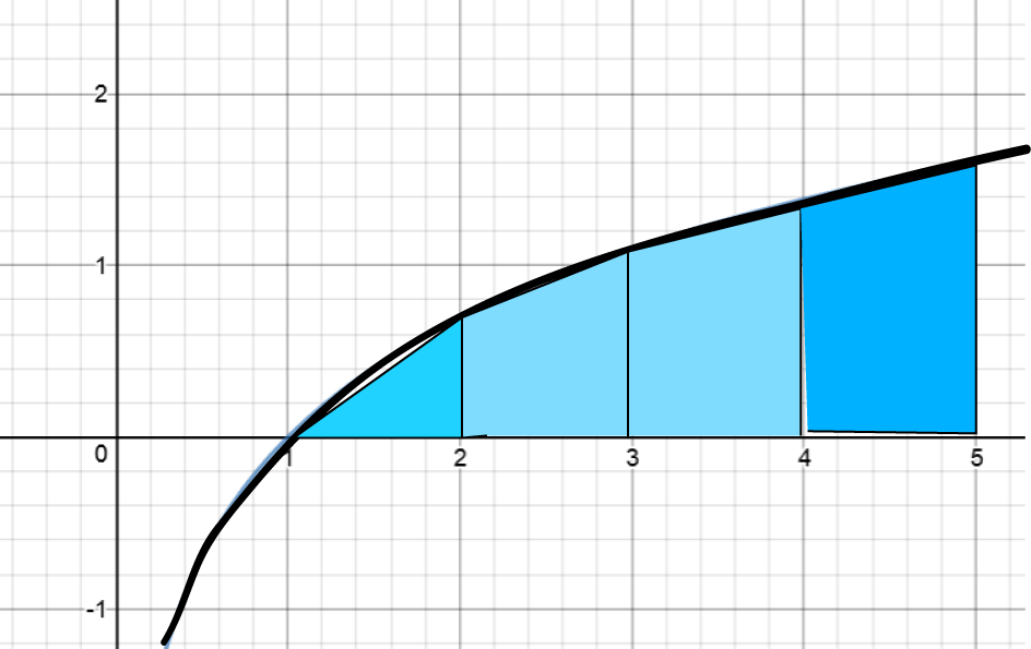
Right Rectangular Approximation Method (LRAM)
This method is also known as the Right Riemann Sum. Funnily enough, this method approximates the area under our curve using
rectangles. The heights of these rectangles are equal to the function values at the right hand end points of each slice, and their widths are equal to
the slice width we chose. Have a look at the picture below to get a better idea of what's going on.
We need to find the areas of each of the \(4\) rectangles in the picture and add them together. This will be our Right Riemann Sum, and
integral approximation.
Let's calculate the areas of those rectangles:
| \(x\)-values | Area Calculation | Area of Rectangle |
|---|---|---|
| 1 - 2 | \(\ln(2) \times 1\) | \(0.6931471806\dots\) |
| 2 - 3 | \(\ln(3) \times 1\) | \(1.098612289\dots\) |
| 3 - 4 | \(\ln(4) \times 1\) | \(1.386294361\dots\) |
| 4 - 5 | \(\ln(5) \times 1\) | \(1.609437912\dots\) |
Adding these all together gives the RRAM approximation of \(4.7874917427\dots\). This is much higher than the actual value of the integral, and if you look at the picture of the rectangles, you can see why. The tops of the rectangles are quite a way above the curve.
Note: Right Riemann Sums will always provide over-estimates for areas under increasing curves. If the curve does some to-ing and fro-ing between increasing and decreasing, some of these errors will cancel each other out, and the approximation will be better.
Midpoint Rectangular Approximation Method (LRAM)
This method is also known as the Midpoint Riemann Sum. Funnily enough, this method approximates the area under our curve using
rectangles. The heights of these rectangles are equal to the function values at the midpoints of each slice, and their widths are equal to
the slice width we chose. Have a look at the picture below to get a better idea of what's going on.
 .
.
We need to find the areas of each of the \(4\) rectangles in the picture and add them together. This will be our Midpoint Riemann Sum, and
integral approximation.
Let's calculate the areas of those rectangles:
| \(x\)-values | Area Calculation | Area of Rectangle |
|---|---|---|
| 1 - 2 | \(\ln(1.5) \times 1\) | \(0.4054651081\dots\) |
| 2 - 3 | \(\ln(2.5) \times 1\) | \(0.9162907319\dots\) |
| 3 - 4 | \(\ln(3.5) \times 1\) | \(1.252762968\dots\) |
| 4 - 5 | \(\ln(4.5) \times 1\) | \(1.504077397\dots\) |
Adding these together gives the MRAM approximation of \(4.07859620525\dots\), which is pretty close to the actual value of \(4.04718956210502\dots\)
Trapezoidal Rule
This rule approximates the area under the curve by adding up the areas of trapeziums. One trapezium is based on each chunk that we've divided the interval \([1,5]\) into. The heights of the parallel sides of the trapeziums are given by the function values at the left and right had end points of each subinterval. The total area is actually equal to the average of the LRAM and the RRAM for the integral.
Let's calculate the areas of those trapeziums (technically, if you want to sound very learned, you should say "trapezia"):
| \(x\)-values | Area Calculation | Area of Trapezium |
|---|---|---|
| 1 - 2 | \(\dfrac{\ln(1)+ \ln(2)}{2} \times 1\) | \(0.3465735903\dots\) |
| 2 - 3 | \(\dfrac{\ln(2)+ \ln(3)}{2} \times 1\) | \(0.8958797346\dots\) |
| 3 - 4 | \(\dfrac{\ln(3)+ \ln(4)}{2} \times 1\) | \(1.242453325\dots\) |
| 4 - 5 | \(\dfrac{\ln(4)+ \ln(5)}{2} \times 1\) | \(1.497866137\dots\) |
Adding these together gives the trapezoidal approximation of \(3.982772786\dots\), which is a bit lower than the actual value of \(4.04718956210502\dots\). The trapezoidal rule tends to underestimate the areas under functions that are concave down.
Did you see how each function value was used twice in the trapezoidal rule calculation? We can write down a general formula for the trapezoidal rule when we divide our interval up into \(n\) equal sub-intervals of width \( h\) as follows:
One last thing to note is that the trapezoidal rule gives an approximation that is the average of the Left and Right Riemann sums.
Simpson's Rule
Simpson's Rule provides a better approximation than the Trapezoidal Rule for the areas under curves that are shaped a bit like polynomials. It uses the areas under parabolas to approximate the area under the function on each sub-interval. It sounds like the formula must be very complicated, but really, three function values are enough to nail down a parabola, so it isn't much more complicated than the Trapezoidal Rule formula. The formula requires an even number of subdivisions of the interval that we are integrating over. If the width of each sub-interval is \(h\) and there are \(n\) subintervals, then the Simpson's Rule approximation can be calculated using the following formula:
 .
.
I did a Simpson's Rule approximation to our integral with \(2\) slices of width \(2\), and came up with the approximation \(4.00259137807\dots\), which isn't as good as the MRAM approximation, but I used wider panels. An application of Simpson's Rule using \(8\) slices of width \(0.5\) yielded an approximation of \(4.04665506569097\dots\), which is really close to the actual value!
Errors in the Approximations
Let's compare the values of the actual value of our integral and its various approximations for different numbers of subdivisions of the interval \([1,5]\).
| Method | N= 4 Estimate | Error (3 d.p.) | N= 8 Estimate | Error (3 d.p.) | N = 100 Estimate | Error (3 d.p.) |
|---|---|---|---|---|---|---|
| LRAM | \(3.17805383\dots\) | \(-0.869\) | \(3.628325017\dots\) | \(-0.419\dots\) | \( 4.014894144\dots\) | \(-0.032\) |
| RRAM | \(4.787491742\dots\) | \(0.740\) | \(4.433043974\dots\) | \(0.386\) | \( 4.0792716608\dots\) | \(0.032\) |
| MRAM | \(4.078596205\dots\) | \(0.031\) | \(4.0553824522\dots\) | \(0.008\) | \( 4.04724288933\dots\) | \(0.007\) |
| Trapezoidal Rule | \(3.9827727865\dots\) | \(-0.064 \) | \(4.0306844959\dots\) | \(-0.017 \) | \( 4.0470829025\dots\) | \(-0.0001 \) |
| Simpson's Rule | \(4.041476218829\dots\) | \(-0.006\) | \(4.04665506569\dots\) | \(-0.001\) | \( 4.047189534018\dots\) | \(0.000000\) |
Simpson's Rule is definitely the most accurate of the approximations for this function. However, different functions will produce different answers. Why don't you pick your favourite function and see what happens?
Formulas for Error Estimates
As we don't always have an exact value of the integral to compare against, there are formulas for error estimates that come in handy. We won't deal with them in any great depth, but here are the formulas for the maximum error in three of our integral approximations:
| Method | Maximum Error |
|---|---|
| MRAM | \( |E| = \dfrac{K(b-a)^3}{24n^2}\) |
| Trapezoidal Rule | \(|E| = \dfrac{K(b-a)^3}{12n^2}\) |
| Simpson's Rule | \(|E| = \dfrac{M(b-a)^5}{180n^4}\) |
In the formulas above,
- \(|E\) is the size of the maximum error
- The integral is taken over the interval \((a,b)\)
- \(n\) is the number of sub-intervals
- \(K\) is the largest absolute value of the second derivative of the function in the interval.
- \(M\) is the largest absolute value of the fourth derivative of the function in the interval.
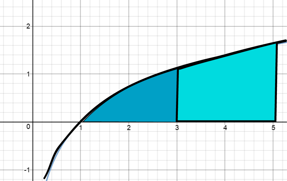
Geometric Shortcuts
Sometimes, part of the area under a curve may correspond to the area of a geometric shape. Rather than approximating the area under that part of the curve, you should find the exact area using well-known geometric formulas. Let's look at some examples.
Triangles
The area under \(y = 4 - x\) from \(x = 0\) to \(x = 4\) is equal to the area of the triangle, \(A = \dfrac{1}{2} \times 4 \times 4\).
Parts of Circles
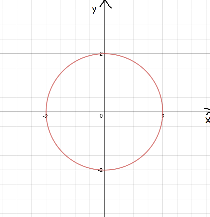
The area under \(y = \sqrt{16 -x^2}\) from \(x = 0\) to \(x = 4\) is equal to the area of a quarter of a circle, \(A = \dfrac{\pi(4)^2}{4} = 4 \pi\).
Rectangles
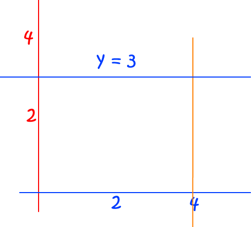
The area under \(y = 3\) from \(x = 0\) to \(x = 4\) is equal to the area of a rectangle, \(A = 3 \times 4 = 12\).
Summary
We can estimate the areas under curves by dividing the interval of integration up into smaller sub-intervals. We obtain better estimates by making smaller subdivisions.
This article has discussed the following five techniques for finding the area under a graph:
- Left Rectangular Approximation Method (LRAM)
- Right Rectangular Approximation Method (RRAM)
- Midpoint Rectangular Approximation Method (MRAM)
- Trapezoidal Rule
- Simpson's Rule
If we don't know the exact value of an integral, there are error formulas that can help us to determine the maximum possible error in the estimates provided by these techniques.
We can sometimes use basic geometric facts to find the areas under some parts of a curve.
Description
Calculus is the branch of mathematics that deals with the finding and properties of derivatives and integrals of functions, by methods originally based on the summation of infinitesimal differences. The two main types are differential calculus and integral calculus.
Environment
It is considered a good practice to take notes and revise what you learnt and practice it.
Audience
Grade 9+ Students
Learning Objectives
Familiarize yourself with Calculus topics such as Limits, Functions, Differentiability etc
Author: Subject Coach
Added on: 23rd Nov 2017
You must be logged in as Student to ask a Question.
None just yet!