Differential Equations

Introduction

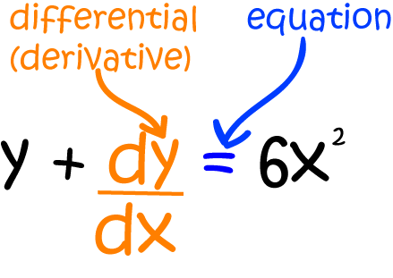
Differential Equations are equations involving a function and one or more of its derivatives.

For example, the differential equation below involves the function \(y\) and its first derivative \(\dfrac{dy}{dx}\).

Solving Differential Equations

Solving differential functions involves finding a single function, or a collection of functions that satisfy the equation.

Not all differential equations can be solved, but there are a number of tricks that can be used to solve equations of certain types.

Let's have a look at some of the different types of differential equations that we can solve. Later articles will show you how to solve separable, some homogeneous and some linear differential equations.

Why does anyone care about differential equations?

Differential equations have many uses in fields such as biology, finance and engineering. We often encounter differential equations when we are trying to descirbe how different things in our world change.

Example (Fruit flies)

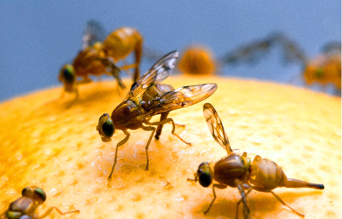You've probably encountered fruit flies before. They're the pesky little things that seem to materialise out of thin air and buzz around the stoned fruit in the summer. Biologists are interested in fruit flies because they breed quickly and easily, and are useful for exploring the transmission of genetic traits.

Biologists are also interested in modelling the growth of populations, and fruit fly populations certainly grow! You need fruit flies to produce more fruit flies, and as you get more fruit flies, the fruit fly population increases more and more rapidly. So, if I want to model the growth of the fruit fly population in and around my fruit bowl, I need to come up with some parameters (variables) for my model. I think the following will be helpful:

• The time, \(t\).
• The number of fruit flies present and any time \(t\). Let's call it \(F\).
• The rate of change of the fruit fly population, \(\dfrac{dF}{dt}\).

Now, I need a few initial values for my model. There seem to be a lot of fruit flies, and they seem to reproduce really rapidly, so let's say:

• The initial population \(F\) is \(1,000\)
• The growth rate \(k\) is 15 new fruit flies per day for every current fruit fly.

Then, the rate of change of my fruit fly population is \(\dfrac{dF}{dt} = 1,000 \times 15 = 15,000 \text{ new fruit flies per day}\). That seems about right, doesn't it? The pesky little things are everywhere!

But that only gives me the population at a specific time. My fruit fly population is constantly, annoyingly, increasing, and I want to model its growth at any time. The better option is to set up a differential equation. We say that the rate of change (at any time) of the fruit fly population is equal to the population's growth rate times the number of fruit flies present at that time:

The above equation is a differential equation because it provides a relationship between a function \(F(t)\) and its derivative \(\dfrac{dF}{dt}\). This particular differential equation expresses the idea that, at any instant in time, the rate of change of the population of fruit flies in and around my fruit bowl is equal to the growth rate times the current population.

Differential equations can be used to model many different things including population growth and decline, radioactive decay, the motion of springs and other bodies, the orbits of spacecraft, the motion of waves, and solar flares. Because they describe rates of change, differential equations are a natural choice of tool to describe many different objects in our universe.

Using Differential Equations

Although they provide a powerful technique for expressing rates of change, differential equations are difficult to use unless we develop methods for finding their solutions. Techniques for solving differential equations often involve applying tricks to reduce the differential equation into a simpler format that no longer involves the derivatives. We can then use the solutions to do calculations, make predictions, draw graphs, and so on. Let's have a look at a few more real-world uses of differential equations.

Compound Interest

When compound interest is applied, the invested (or borrowed) money acts a bit like our fruit flies. You need to invest money to get money, and the more money you have, the more money you end up with. In compound interest, the initial amount of money invested earns interest, but so does the interest on the investment. This interest is calculated after a given time period such as a month, a quarter or a day and added to the original amount.

You may have seen formulae for compound interest in the sequences and series section of your maths textbook. These are the sorts of formulae you get when the interest is added to the original investment monthly or yearly, but when it is continuously calculated and compounded, you need a differential equation to model the equation.

It's time to come up with some parameters for the compound interest model. We need:

• The amount invested, \(P\).
• The interest rate, \(r\).
• The time, \(t\), and
• The rate of change of the amount invested, \(\dfrac{dP}{dt}\)

Just like the fruit flies, the bigger the amount invested, the more interest it earns. We can come up with the following differential equation for the growth of investments whose interest is continually compounded: If you think you've seen this before, you're right. It looks just like the equation we came up with for the fruit flies. Mathematics can't tell money and fruit flies apart! That's because mathematics is only interested in the rates of change of these two things, and not in their physical characteristics.

Solving this equation

Coming up with this differential equation is all well and good, but it's not very useful unless we can solve it. Luckily, this is one of the types of differential equations that can be solved easily. It's an example of a separable differential equation, and we'll talk more about them in another article.

For now, you just need to know that this equation has the following solution:

where \(P_0\) is the principal (or initial amount invested).

Let's have a look at the value of an investment of \(\$2,000\) at an interest rate of \(5\%\), continuously compounded over 3 years:

Further examples of differential equations

The Verhulst Equation and the Carrying Capacity of Environments

Back to Our Fruit Flies

Our original model for the rate of change of the fruit fly population wasn't quite realistic enough because it failed to take into account the fact that a given environment (like my fruit bowl) only has enough food in it to support a certain population. This maximum population that an environment can support is called the carrying capacity of the environment.

A Belgian mathematician, Pierre Francois Verhulst, figured this out in 1838, and his work was later modified by American scientists Raymond Pearl and Lowell Reed to produce the Verhulst equation:

in which \(P(t)\) represents the population at time \(t\), \(r\) is the growth rate and \(K\) is the carrying capacity of the environment. Pretty clever, huh?

Springs and Things

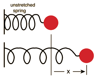Have you ever played with springs in the science lab at school? The English physicist, Robert Hooke had lots of fun with springs back in around 1660. He noticed that the force required to stretch a spring through a distance of \(x\) units from its equilibrium (resting) position was equal to some constant \(k\) times the distance the spring was extended. In other words, he formulated Hooke's law:

At first glance, this doesn't look much like a differential equation, but we're not finished yet! Newton's second law says that if an object of mass \(m\) is attached to the end of the spring, the force is equal to \(m\) times the acceleration of the spring: And \(a = \dfrac{d^x}{dt^2}\). This force has to be equal to the force obtained through Hooke's law. So, we do have a differential equation after all: It's a differential equation of order \(2\) since it involves the second derivative.

Creating a differential equation is just one part of the battle when you're trying to model changes in things in the universe. It's a very important step, but we need to be able to get some numbers out of the differential equation before we can do anything useful with it. If we want to be able to describe the way our spring bounces up and down, we need to solve the differential equation \( m\;\dfrac{d^2x}{dt^2} = -kx\). Getting useful information out of differential equations often involves finding their solutions, although sometimes it may only be possible to come up with approximate solutions.

There are a number of steps that we need to go through before we can solve a differential equation. That is, of course, if it is possible to solve the equation. The first is to classify the equation. This is necessary so that we can identify the appropriate technique for solving the equation, if one exists.

Classifying Differential Equations

Ordinary or Partial

This is the first thing to check:

• Ordinary differential equations (ODEs) involve only one independent variable and its derivative, e.g. \(y\) and \(\dfrac{dy}{dx}\).
• Partial differential equations (PDEs) involve two or more independent variables and their partial derivatives.

We're only interested in ordinary differential equations in this article.

Order and Degree

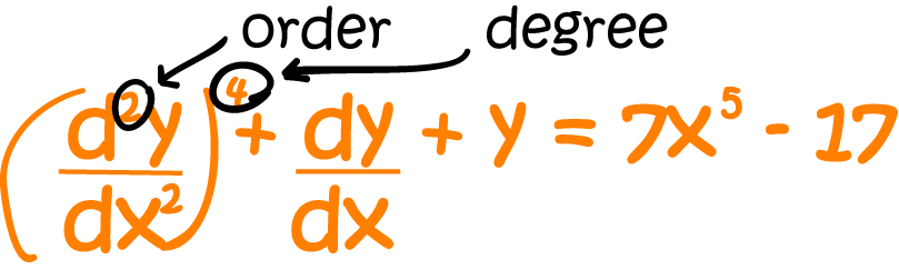
The order is the next most important thing to check. It is the highest derivative (first, second, third,...) involved in the equation. The above equation includes a second derivative, so it has order \(2\).

The degree is also important. It's the highest power of the highest derivative involved in the equation. In the above example, the degree is \(4\) - there's a term in \(\left(\dfrac{d^2y}{dx^2}\right)^4\).

Let's look at a few more examples:

Example:

involves only a first derivative, so it has order 1. It has degree \(1\) because the highest power of \(\dfrac{dy}{dx}\) involved is \(1\), so it is a first order, first degree ordinary differential equation.

Example:

has order \(2\) and degree \(3\), so it's a second order, third degree ordinary differential equation.

Example:

has order \(3\) and degree \(1\). The power \(4\) of \(\dfrac{dy}{dx}\) doesn't count because the highest order derivative is \(\dfrac{d^3 y}{dx^3}\).

Type of Differential equation

There are many different types of differential equations, but we shall focus on three main types:

1. Separable differential equations like \( x \dfrac{dy}{dx} = \cos^2(y)\).
2. First order linear differential equations. These look like:
   \( \dfrac{dy}{dx} + P(x) y = Q(x). \)
   Linear refers to the fact that they include only the linear function \(y\), and not any other function of \(y\).
3. Homogeneous differential equations. These look like:
   \( \dfrac{dy}{dx} = f(x,y), \)
   where \(f(x,y)\) is a homogeneous function in the sense that \(f(tx,ty) = f(x,y)\) for all values of \(t,x,\) and \(y\).

Have a look at the articles on these three types of ordinary differential equations to learn how to solve them.