Calculus
Chapters
Introduction to Integration
Introduction to Integration
There are many different uses for integrals. These include finding volumes of solids of revolution, centres of mass, and the distance that Gus the snail has travelled during his attempts on the land-speed record. Integrals also have many applications in Physics. One common use of integrals is to find the area under the graph of a function.
Finding these Areas
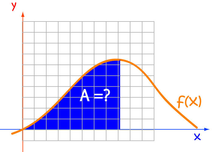
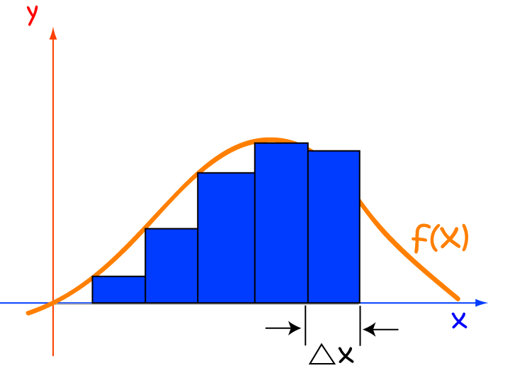
An integral is a giant sum. To find the area under the graph of a function, we begin by splitting the \(x\)-axis up into little chunks, and then add up the areas of rectangles based on these chunks. You might see these little rectangles called slices in some books.
Finding the Limit of this Sum
Fortunately, we usually don't actually have to find this sum and take the limit. That is, unless your calculus teacher or an exam question asks you to, or if there's a reason why we can't find the integral in another way! To find out more about this, see the article on integral approximations.
Most of the time, there's a handy short cut we can use. This is because integrals are just the opposite of derivatives. If we
can work out what function has been differentiated to give \(f(x)\) (sometimes called a primitive function or an anti-derivative),
then we know what \(\displaystyle{\int f(x) \; dx}\) is equal to.
Example:
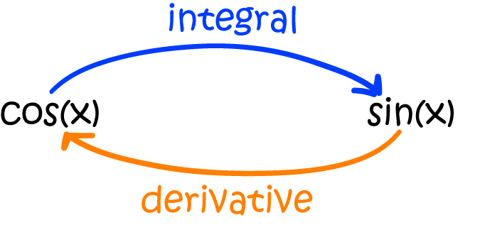
What is the integral of \(\cos(x)\)?
We know that the derivative of \(\sin(x)\) is \(\cos(x)\) ...
and someone said that integrals and derivatives are opposites ...
so an integral of \(\cos (x)\) is \(\sin (x)\).
Anatomy of an Integral
The symbol for an integral looks a bit like an elongated "S". Think of this as "S" for sum. Don't forget that
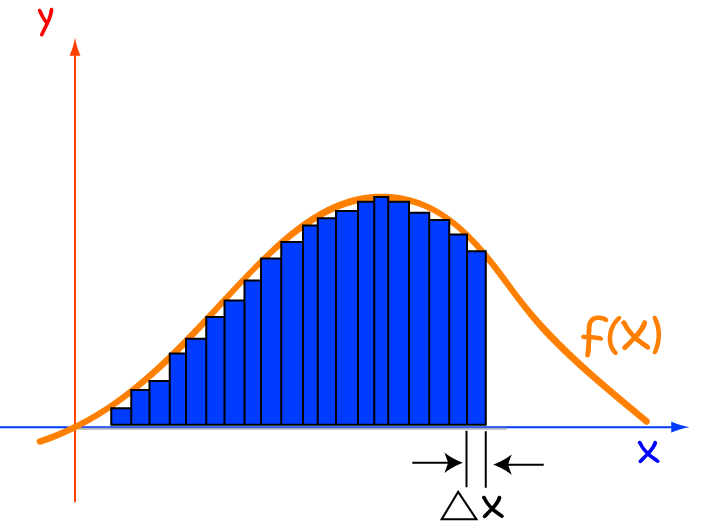
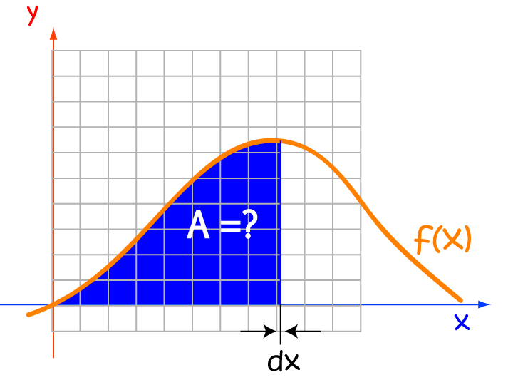
we are adding up rectangles, based on the \(x\)-axis, whose width \(\Delta x\) tends to \(0\). We write
this as \(dx\). The other parts of the integral are shown in the diagram
below:
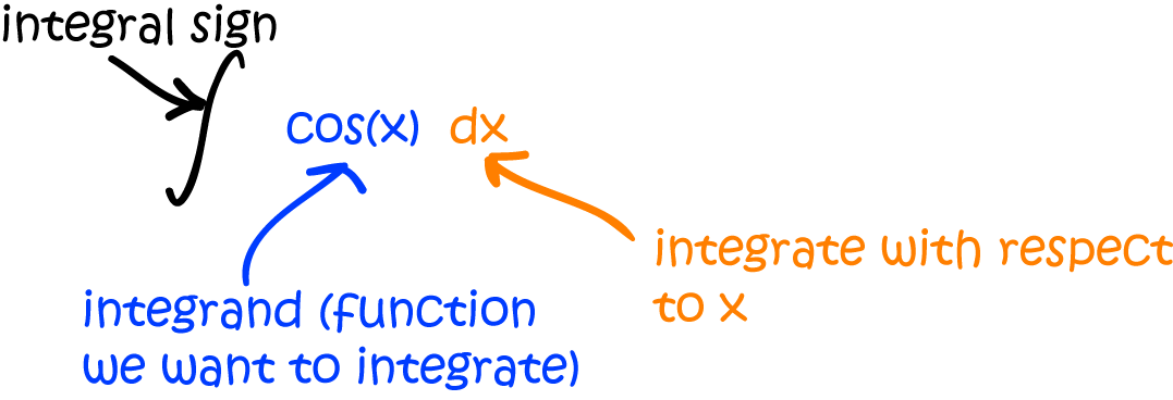
Note that the integrand (the function we're integrating) is placed immediately after the integral sign, and the whole thing is finished off with a \(d\text{(variable of integration)}\) to indicate that we're integrating with respect to this variable. Of course, this variable needn't be an \(x\): it could be anything you like. For example, Gus the snail might think of writing:
Back to our Example
We can now use our new notation on our example. Remember, we were asked to find the integral of \(\cos(x)\), and we know that the derivative of \(\sin(x)\) is \(\cos (x)\). Here's the way we write the answer:
What's this C thingy at the end?
We call \(C\) the constant of integration. The point is that there are zillions of functions that you can differentiate
to give \(\cos(x)\) (infinitely many, in fact). This is because the derivative of a constant is zero. Here are some of them:
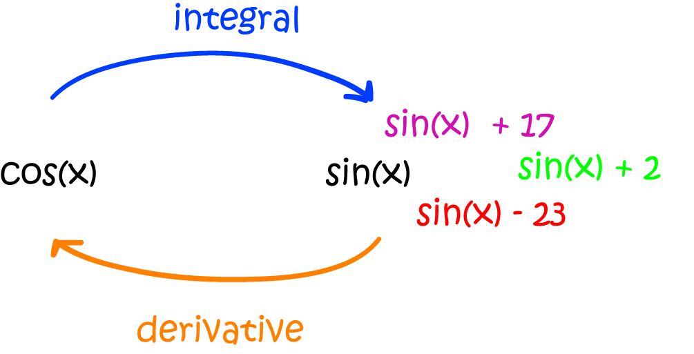
So, performing the reverse of differentiation only tells us what part of the answer is. We need to indicate the whole family of answers that are possible by adding the constant \(C\). Of course, there's no real reason why we call the constant \(C\). You could just as correctly call it Murgatroyd to give
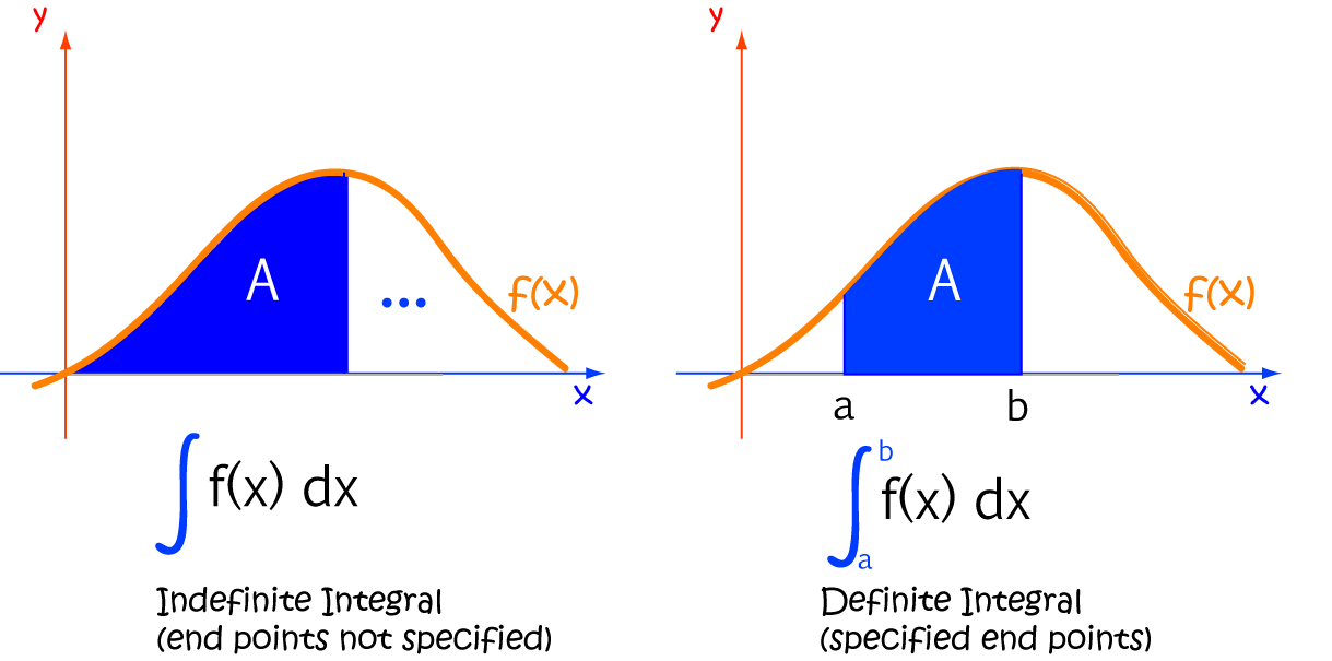
Definite Integrals
As opposed to indefinite integrals, definite integrals have beginning and end values that decorate the integral sign. The bottom value indicates the beginning of the interval, and the value up the top indicates the end value.
Have a look at the article on definite integrals for more information about these handy animals.
Speed and Distance
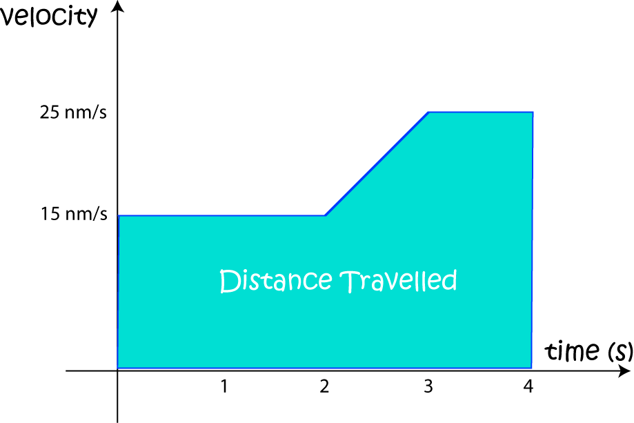
Remember Gus the snail? He's in training to beat the world land-speed record. He's put together the following graph of his velocity and wants to know the total distance he's covered during training.
What's this have to do with integrals? I'm glad you asked.
Gus' velocity is the rate at which he adds distance to his total distance travelled. At each instant of his training, he adds a tiny little rectangle of width \(dt\) and height \(v(t)\) to the area under the curve. We integrate the velocity (add up all the areas of the rectangles) to find the total distance he has travelled. As Gus glides faster, the distance he has travelled increases more quickly. We integrate the velocity function to get the distance travelled.
The reverse is true as well. If we know the distance function, we can work out the velocity function. It's equal to the derivative of the distance function.
We can work out the area under Gus' velocity curve quite easily. Split the area up into a rectangle (for times between \(0\) and \(2\) seconds), a trapezium (for times between \(2\) and \(3\) seconds), and another rectangle (for times between \(3\) and \(4\) seconds). Then the distance (area under the curve, or definite integral) is given by:
This also gives us a nice reason for the need for the \(C\) in the indefinite integral. If Gus had already travelled a certain distance before he started to record his velocities, we could add that distance onto the distance he travelled after he started recording the velocities.
That's enough about definite integrals for now. Let's calculate a few more indefinite ones. A lot of the reverse differentiation has already been done for us. See the article on integration rules for some of the details. You can also read the differentiation rules backwards!
Example
The table in the rules of derivatives article tells us that the derivative of \(\tan(x)\) is \(\sec^2(x)\). So
Are you ready for another one?
Example
The integration rules page gives us a "power rule" for integration. It says:
Conclusion
The key to being good at integration is learning the various integration rules and techniques, and then getting lots of practice. Keep it simple at first. Try evaluating a few simple integrals of each type. You can either get examples out of a book, or make them up yourself. Don't try to be too clever and make them complicated. Be warned that there are some functions like \(f(x) = e^{x^2}\) that don't have any anti-derivatives. Just integrate one basic function at a time. Once you've mastered basic integration, you can move on and read the articles on integration by substitution and integration by parts.
Description
Calculus is the branch of mathematics that deals with the finding and properties of derivatives and integrals of functions, by methods originally based on the summation of infinitesimal differences. The two main types are differential calculus and integral calculus.
Environment
It is considered a good practice to take notes and revise what you learnt and practice it.
Audience
Grade 9+ Students
Learning Objectives
Familiarize yourself with Calculus topics such as Limits, Functions, Differentiability etc
Author: Subject Coach
Added on: 23rd Nov 2017
You must be logged in as Student to ask a Question.
None just yet!