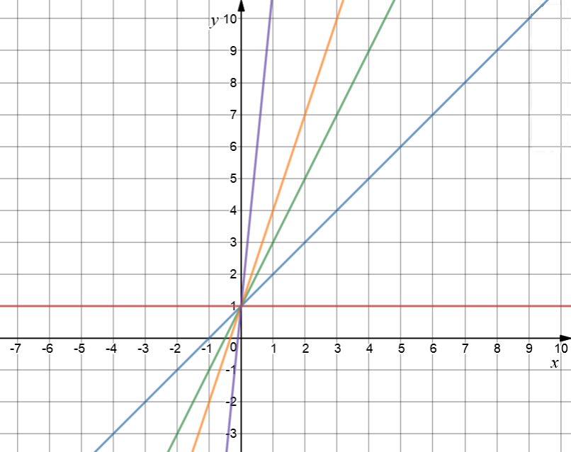
Let's see what happens to the line if we change the values of \(m\) to different non-negative integers. The red horizontal line has equation \(y=1\). The gradient is equal to zero. Next we'll increase the gradient to \(1\) to give the blue line \(y = x + 1\). A gradient of \(2\) produces the green line \(y = 2x + 1\), and a gradient of \(3\) produces the orange line \(y = 3x + 1\). Now let's go completely crazy! A gradient of \(10\) produces the purple line, \(y = 10x + 1\).

What happens to the line as I increase the gradient (notice that I've kept everything else the same)? The line gets steeper and steeper. It goes from horizontal, when \(m= 0\) to really quite steep when \(m = 10\). I can never make it exactly vertical by changing the value of \(m\), but I can make it as close to vertical as I like. Why not have a play around on an on-line graphing calculator with different values of \(m\) and see what you get?

Now I'm going to see what happens if I change the values of \(m\) between \(0\) and \(1\). I got a bit bored with my \(b\)-value, so I changed it to \(2\). Here we go. Hold on to your hats!

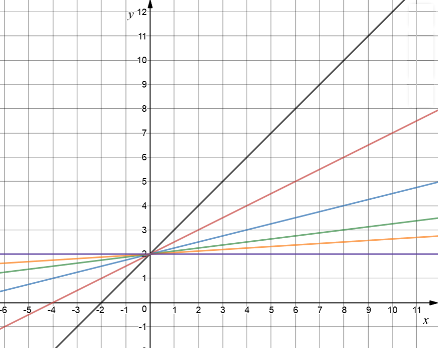
If \(m=1\), I get the black line \(y = x + 2\). The red line is \(y = 0.5 x + 2\). I've taken the extremely dangerous step of changing the gradient to \(0.5\). Next, we have \(y = 0.25 + 2\) in blue, with \(m = 0.25\), followed by the green \(y = 0.125x + 2\), where \(m = 0.125\). In orange, we have \(y = 0.0625x + 2\), and the horizontal purple line has \(m = 0\). It is \(y = 2\).

As \(m\) decreases in value between \(1\) and \(0\), the line flattens out. It becomes flatter as \(m\) edges closer to \(0\), and is finally completely flat for \(m = 0\).

There's one thing left to explore. What happens if we make \(m\) negative?

Well, for a start, \(m\) slopes backwards. Instead of the graph going uphill as we move from left to right, it goes downhill.

The slope depends on the absolute value of \(m\). As the absolute value of \(m\) increases, the lines get steeper, but they're going downhill rather than uphill.

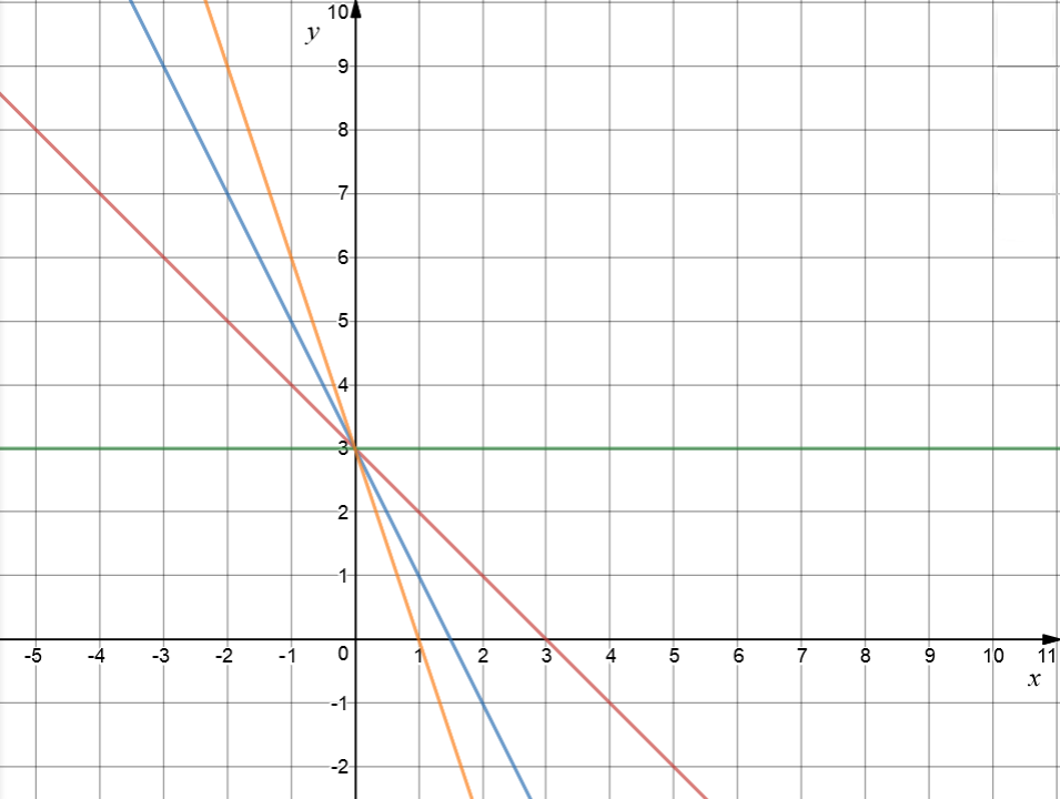
I keep getting bored with my \(b\)-values, so I've changed \(b\) to \(3\) this time. I have drawn the horizontal line \(y = 3\) in green. \(y = -x + 3\) is in red, with its slope of \(-1\). This is followed by \(y = -2x + 3\) in blue (gradient \(-2)\), and \(y = -3x + 3\) in orange (\(m = -3\)). As the absolute value of \(m\) gets larger, the slope gets steeper.

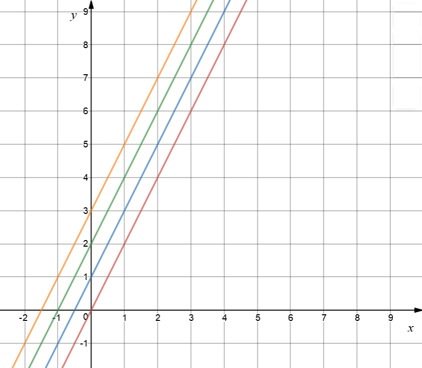
This delightful collection of graphs all have gradients of \(2\). First up, looking charming in red, we have the graph of \(y = 2x\). It only cuts the \(y\)-axis at \(y = 0\), so its \(b\)-value is \(0\). Next is the stunning graph of \(y = 2x + 1\) in blue. It cuts the \(y\)-axis at \(y = 1\). Moving along, we have the very dapper \(y = 2x + 2\) in green, with a \(y\)-intercept of \(2\). We'll finish with the dashing \(y = 2x + 3\), bedecked in orange. Who would have believed what a \(y\)-intercept of \(3\) could do to a graph.

Seriously though, do you notice how all of these graphs are parallel to each other? They've just been shifted further up the \(y\)-axis as the values of \(b\) are increased.

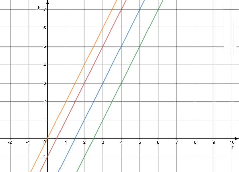
Finally, let's play with some negative values of \(b\). I've kept the gradient (\(m\)) equal to \(2\), so they're all parallel. Negative \(b\)-values cause the graph to slide down the \(y\)-axis.

The orange graph is \(y = 2x\). I've just included a graph with a \(b\)-value of \(0\) as a reference. The red graph is \(y = 2x - 1\). It's been shifted one unit down the \(y\)-axis because it has \(b = -1\). Next, the blue graph is \(y = 2x - 3\), parallel to the others, but shifted \(2\) units further down the \(y\)-axis, by making \(b = -3\). Finally, the green graph is \(y = 2x - 5\). It is still parallel to the others, but shifted down even further by its value of \(b\), which is \(-5\).