Data
Chapters
Standard Deviation and Variance
Standard Deviation and Variance
Standard Deviation measures how spread out the values in a set of data are. We use the Greek letter \(\sigma\) (sigma) as the symbol
for standard deviation, and calculate it by taking the square root of the variance of the data set.
That's about as helpful as those dictionary definitions that tell you that "integration is the act of integrating something", unless I tell you how to calculate the variance of a data set.
Variance
Variance is the square of the standard deviation (just joking!). The variance of a data set is defined to be the
There are three simple steps to follow to calculate the variance:
- Find the mean (average) of the values
- Subtract each value from the mean and square the result to give the squared difference.
- Find the averages of the squared differences. That's the variance.
- Take the square root to give the standard deviation.
Before we work through an example, let's talk about why we square the differences.
So, Why Do We Square the Differences?
I'm glad you asked!
We square the differences because we want to measure the spread of the data.
Our data values can be above and below the mean, so we end up with positive and negative differences that cancel each other out if we just take the data values as is.
For example, if we just used the differences, and they were \(\{2,-2,2,-2\}\), their mean is \(\dfrac{2 + (-2) + 2 + (-2)}{4} = \dfrac{0}{4} = 0\), which is rubbish as it suggests that the data is not spread out at all.
If we took absolute values of these differences, instead of squaring, we get another measure of spread, which is the mean deviation, but even this has some problems. For example, the mean deviation of the data set with differences \(\{2,-2,2,-2\}\) is \(\dfrac{2 + |-2| + 2+ |-2|}{4} = 2\), and the mean deviation of the data set with differences \(\{3,1,-4,0\}\) is also \(2\), but this set is much more spread out, so this isn't a great measure of the spread of data, either.
Squaring the differences, finding their mean and then taking the square root gives the following values for these two data sets:
- Differences \(\{2,-2,2,-2\}\): \(\sqrt{\dfrac{2^2 + (-2)^2 + 2^2 + (-2)^2}{4}} = \sqrt{4} = 2\)
- Differences \(\{3,1,-4,0\}\) : \(\sqrt{\dfrac{3^2 + 1^2 + (-4)^2 + 0^2}{4}} = \sqrt{\dfrac{26}{4}} = 2.55\)
It looks like squaring the differences and taking the square root of their mean gives a better measure of the spread of the data.
A Worked Example
Sam wants to enter Lucy (our Cavalier King Charles Spaniel puppy) in agility races when she gets bigger. He wants to see how quickly she can run, compared to other dogs, so he asks his friends how quickly their dogs can run. Here are his results.
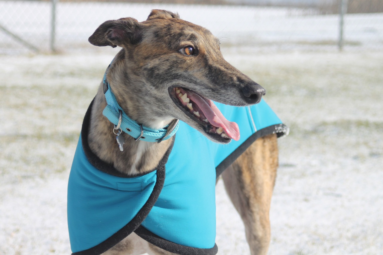
Grace, the greyhound, is pretty speedy. Her top speed is \(64.7\) km/h.
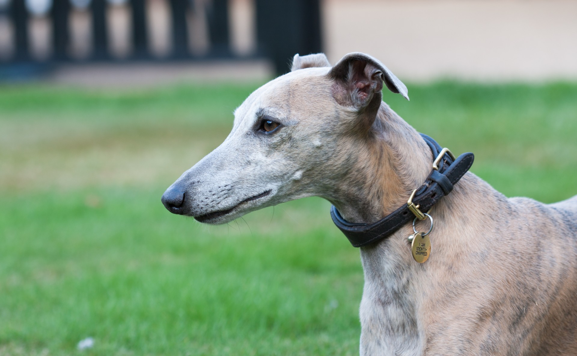
Rosie, the whippet, isn't quite as fast, but she's close. Her top speed is \(64\) km/h.
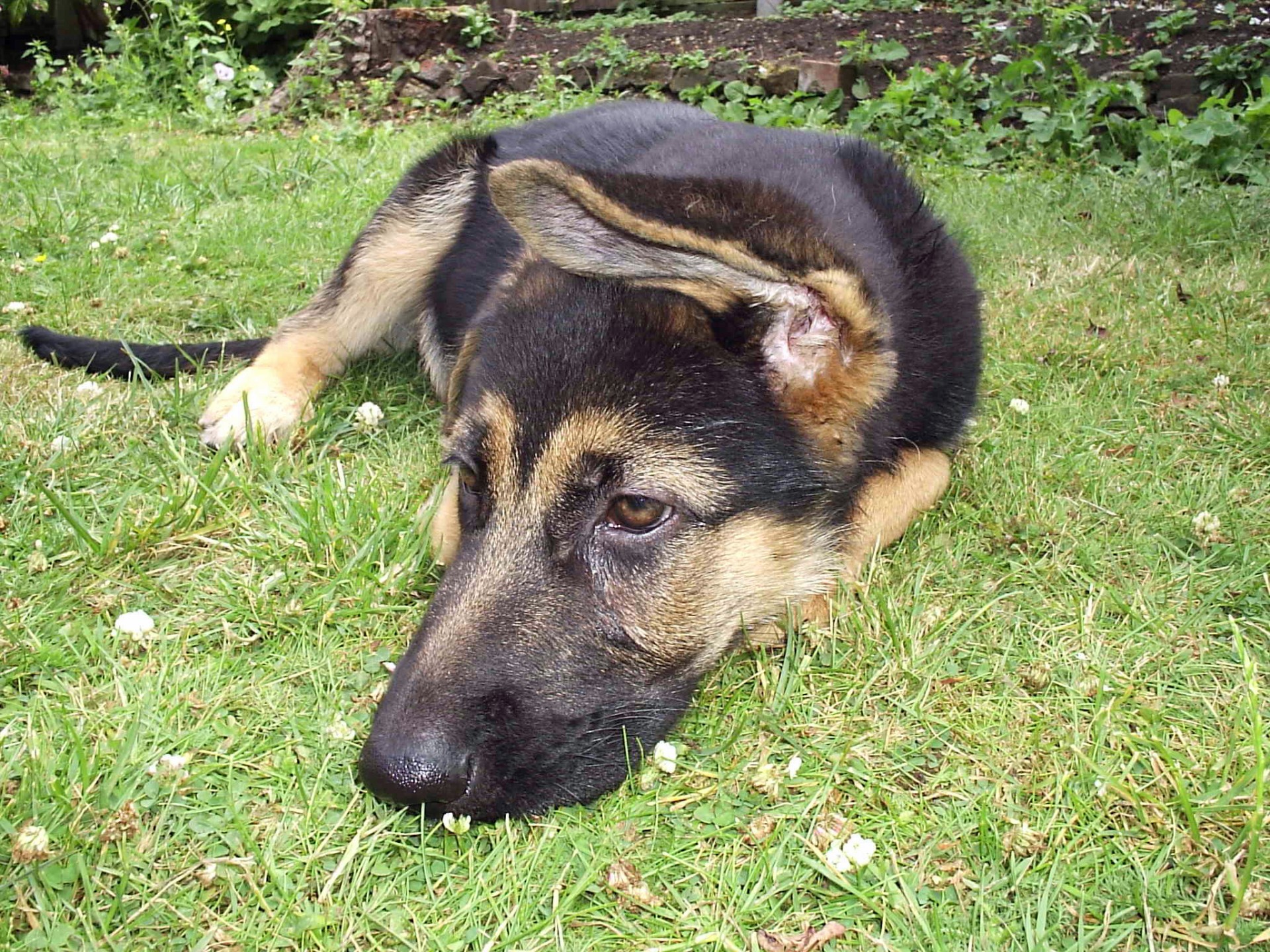
Jackson doesn't look very fast here, but appearances can be deceiving. He's a German Shepherd with a top speed of 63.4 km/h.
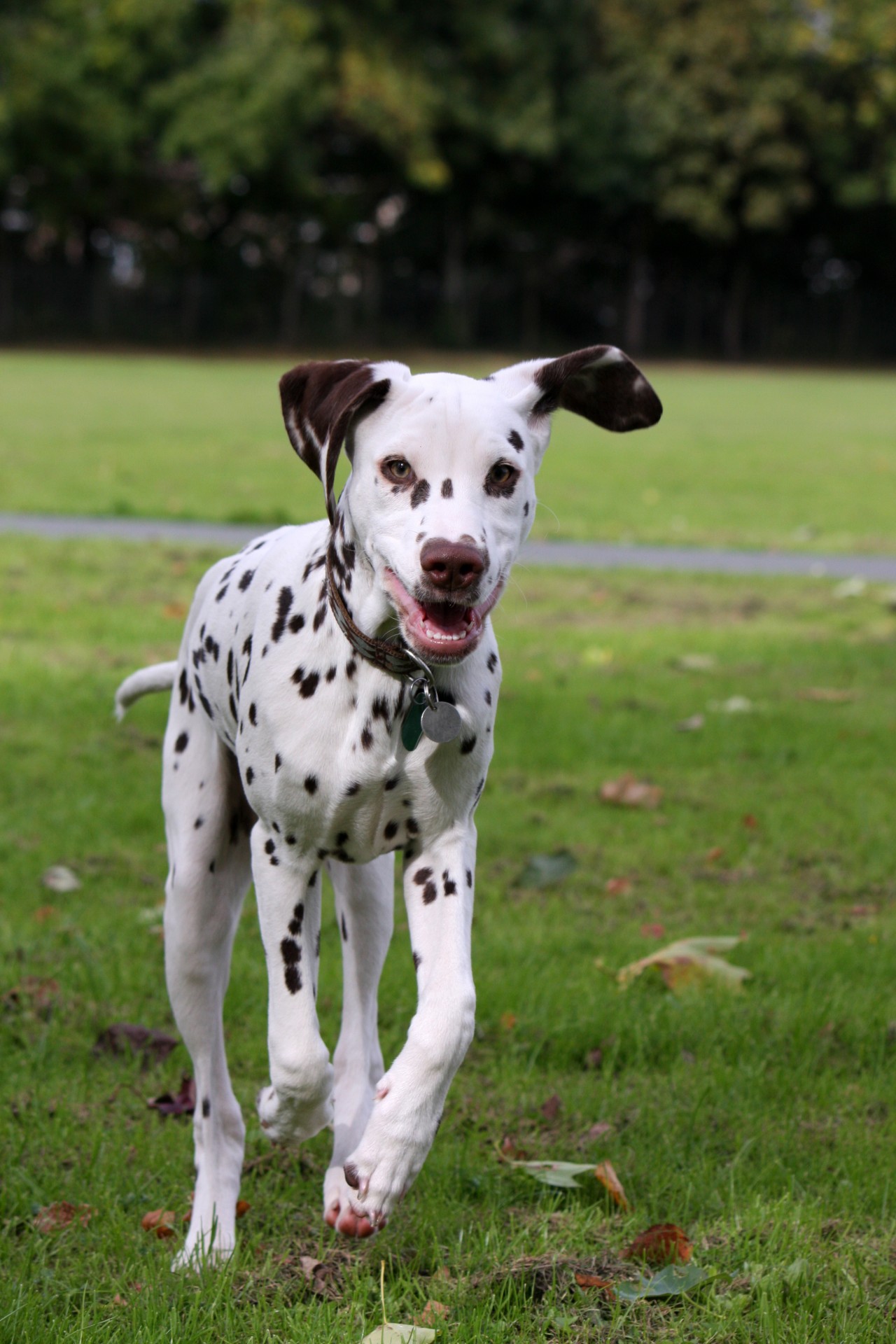
Hunter, the dalmatian puppy, loves to run. His top speed is \(59.5\) km/h.
All of those dogs were pretty big. How about some smaller ones?
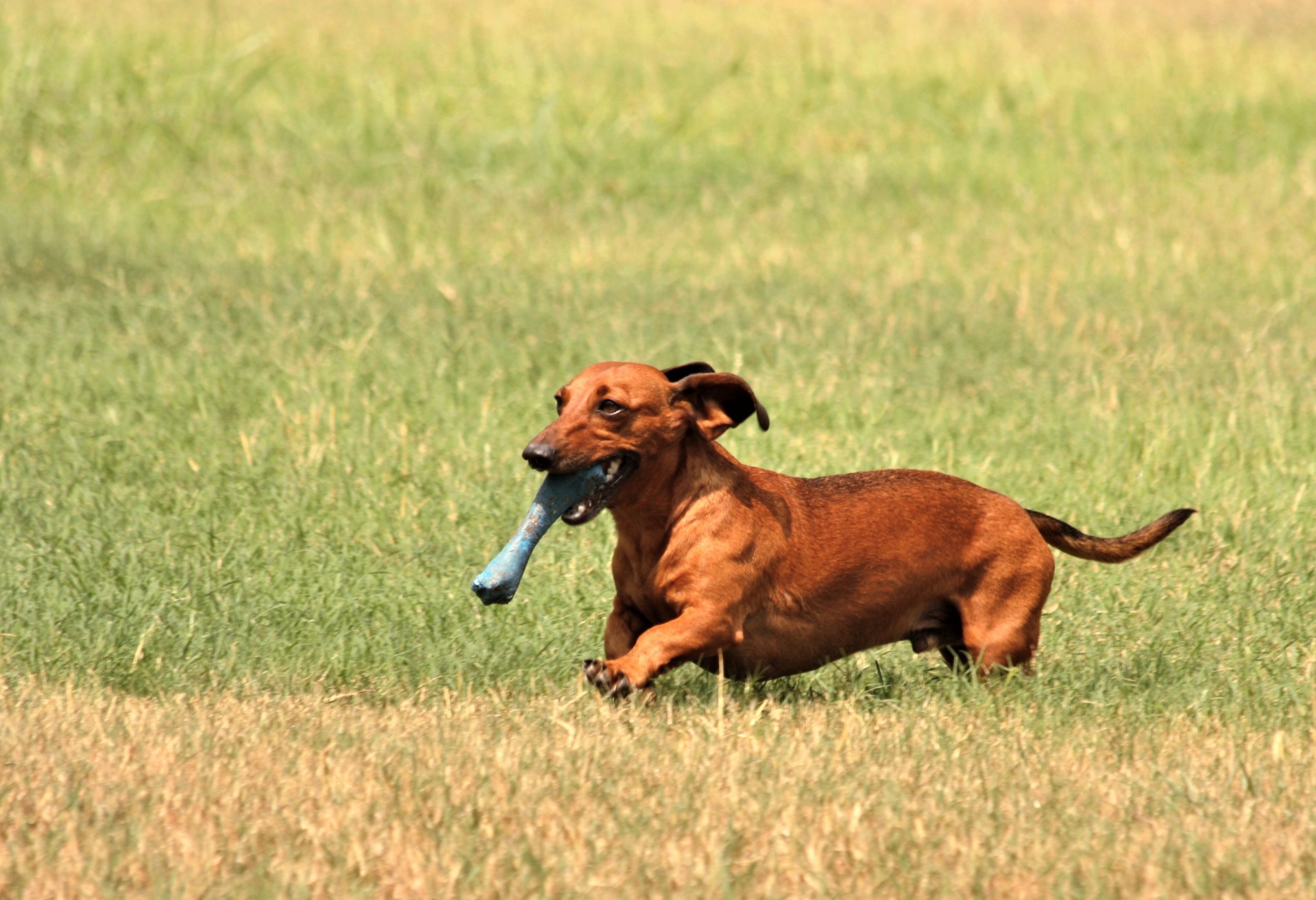
Sausage, our dachshund, only has little legs (don't tell him I said that), but he can move! His top speed is \(31\) km/h.
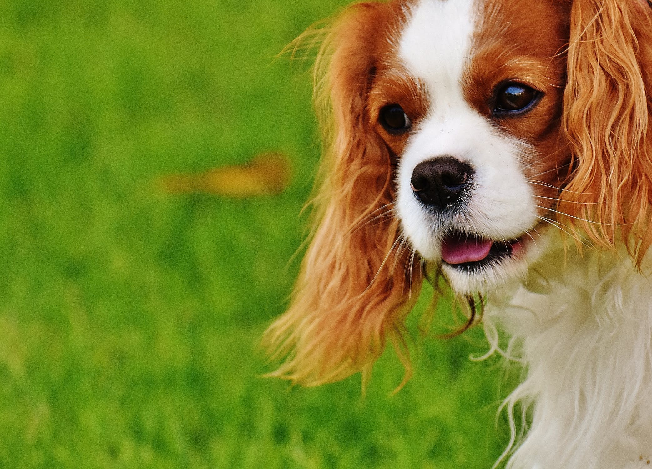
Lucy is still only a puppy, so she'll get faster as her legs grow. Her top speed is \(26\) km/h.
Now let's find the mean, variance and standard deviation of these speeds.
First, the mean:
Next we calculate each doggy's difference from the mean:
- Grace: \(64.7 - 51.43 = 13.27\)
- Rosie: \(64 - 51.43 = 12.57\)
- Jackson: \(63.4 - 51.43 = 11.97\)
- Hunter: \(59.5 - 51.43 = 8.07\)
- Sausage: \(31 - 51.43 = - 20.43\)
- Lucy: \(36 - 51.43 = -25.43\)
The variance is the mean of the squares of these values. So, square each difference, and then find the average of these squares:
To find the Standard Deviation, we just take the square root of the variance to give:
Standard Deviation and Samples
In the example above, we worked with a population of 6 dogs - we were only interested in the 6 dogs that we had data for.
If we want to use the 6 dogs as a sample (a small section of the population that is chosen to represent it), we need to change our formulas slightly.
Instead of dividing the sum of the squares of the differences from the mean by \(N\) (the size of the population) when calculating the variance, we divide it by \(N-1\).
So, if our six dogs is considered to be a sample, we have
The reason for this small change in the formula is that we are trying to correct for differences that might arise between the entire population and the sample.
Conclusion
You can use the steps discussed in the article to calculate the variance and standard deviation of any numerical data set.
Of course, sometimes it is more convenient to have formulas for these measures. We'll talk about those in the article on formulas for standard deviation and variance.
Description
This chapter series is on Data and is suitable for Year 10 or higher students, topics include
- Accuracy and Precision
- Calculating Means From Frequency Tables
- Correlation
- Cumulative Tables and Graphs
- Discrete and Continuous Data
- Finding the Mean
- Finding the Median
- FindingtheMode
- Formulas for Standard Deviation
- Grouped Frequency Distribution
- Normal Distribution
- Outliers
- Quartiles
- Quincunx
- Quincunx Explained
- Range (Statistics)
- Skewed Data
- Standard Deviation and Variance
- Standard Normal Table
- Univariate and Bivariate Data
- What is Data
Audience
Year 10 or higher students, some chapters suitable for students in Year 8 or higher
Learning Objectives
Learn about topics related to "Data"
Author: Subject Coach
Added on: 28th Sep 2018
You must be logged in as Student to ask a Question.
None just yet!