Probability
Chapters
Probability: Tree Diagrams
Probability: Tree Diagrams
Tree diagrams provide you with a way of keeping track of probability calculations. They help you to decide whether you need to add or multiply probabilties to find your desired result. They also have an in-built way of checking whether your calculations are correct.
Let's start by thinking about the problem of drawing a tree diagram to model drawing balls out of a bag.
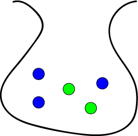
A bag contains 3 blue balls and 2 green balls. The probability of drawing a blue ball out of the bag (without looking) is \(\dfrac{3}{5} = 0.6\), and the probability of drawing a green ball out of the bag (without looking) is \(\dfrac{2}{5} = 0.4\).
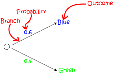
On the right is a tree diagram for drawing a ball out of this bag.
The tree has two branches: one for drawing a blue ball, and the other for drawing a green ball out of the bag.
Each branch is labelled with the probability of taking that branch.
The outcome (Blue or Green) is written at the end of each branch.
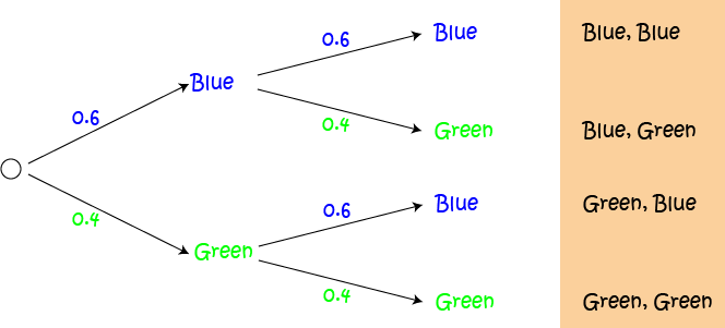
We can extend our tree diagram to model the outcomes of drawing two balls out of the bag. One ball is drawn, and then put back into the bag. The second ball is
then drawn. We call this drawing with replacement because the drawn ball is replaced into the bag after each draw. Here is
our extended tree diagram:
Now we need to calculate the probabilities for each of the listed outcomes.
- We multiply probabilities along the branches leading to each outcome.
- We add probabilities going down the columns of the tree.
Here is the tree with all probabilities calculated:
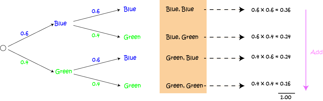
So we can now see that:
- The probability of drawing a green ball, followed by a green ball is \(0.16\).
- The probability of drawing a green ball, followed by a blue ball is \(0.24\).
- The probability of drawing a green ball and a blue ball in any order is \(0.24 + 0.24 = 0.48\) (We added the probabilities for Green followed by Blue and Blue followed by Green)
- All of the probabilities add up to \(1.0\). This helps you to check that you got your sums right.
- The probability of drawing at least one blue ball is \(0.36 + 0.24 + 0.24 = 0.84\).
- And many other things.
This example shows that tree diagrams are great for modelling the probabilities of independent events (because we replaced the ball after
each draw, the outcome of the second draw was independent of the outcome of the previous draw).
In the next example, we shall see that tree diagrams are also useful for modelling the probabilities of dependent events (ones where the
probability depends on the outcome of the previous event). Let's go snail racing with Gus and Alyce!
Example: Gus and Alyce
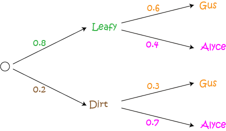
Our neighbourhood speed demons, Gus the snail and his friend, Alyce, are having a race. Their friend, Christo is acting as the referee. The outcome of the race depends on the course chosen, and that is up to Christo.
There are two tracks that Christo can choose for the race. His favourite track is the leafy track, which he chooses with probability 0.8.
Gus has different probabilities of winning the race, depending on the track chosen:
- His probability of winning on the leafy track is 0.6
- His probability of winning on the dirt track is 0.3
What is the probability of Gus winning the race?
This example includes dependent events because the probability of Gus winning depends on which track Christo chooses. Let's build a tree diagram for this example. We begin with the two tracks that Christo might choose:
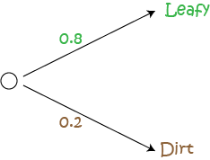
Because there are only two tracks to choose from, and Christo chooses the leafy track with probability 0.8, the probability of him choosing the dirt track is \(1 - 0.8 = 0.2\). Probabilities always add up to 1.
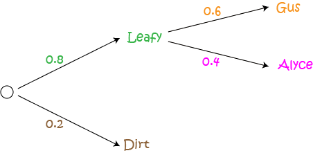
Now, if the leafy track is chosen, Gus has probability 0.6 of winning. So, the probability of Alyce winning on the leafy track is \(1 - 0.6 = 0.4\). Let's fill those probabilities in on the diagram:
What if the dirt track is chosen? Gus has probability 0.3 of winning there, so Alyce wins with probability \(1 - 0.3 = 0.7\). Let's fill in the rest of the diagram:
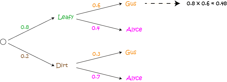
Now we can use our diagram to calculate the probabilities of Gus winning on each track. Follow the branches through to each outcome corresponding to a winning for Gus, and multiply the probabilities that appear on the branches on your path.
The probability of the leafy track being chosen and Gus winning is given by
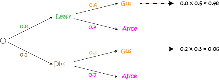
The probability of the dirt track being chosen and Gus winning is given by
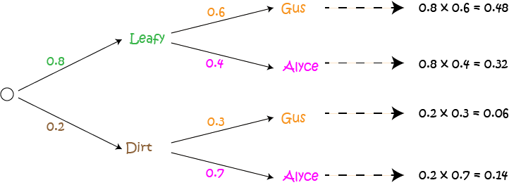
Now, we add the values that we have calculated in our column:
Checking Our Work
We can check our work by calculating the other probabilities (i.e. of Alyce winning) and making sure that all the probabilities sum to 1:
Conclusion
Tree diagrams are useful for keeping track of probability calculations.
We multiply probabilities along the branches of a tree diagram, and add them down the columns.
A useful check is to make sure that all your probabilities add up to 1.
Description
In this mini series, you will learn a bit more on the topic of probability, we will cover topics such as
- Ratios
- Fair dice
- Conditional probability
- Mutually exclusive events
and more
Audience
Year 10 or higher students
Learning Objectives
Explore more on the topic of probability
Author: Subject Coach
Added on: 28th Sep 2018
You must be logged in as Student to ask a Question.
None just yet!